Smoking Prevalence Notebook for Sharing
Libraries
library(tidyverse)## Registered S3 methods overwritten by 'ggplot2':
## method from
## [.quosures rlang
## c.quosures rlang
## print.quosures rlang## -- Attaching packages ---------------------------------------- tidyverse 1.2.1 --## v ggplot2 3.1.1 v purrr 0.3.2
## v tibble 2.1.3 v dplyr 0.8.1
## v tidyr 0.8.3 v stringr 1.4.0
## v readr 1.3.1 v forcats 0.4.0## -- Conflicts ------------------------------------------- tidyverse_conflicts() --
## x dplyr::filter() masks stats::filter()
## x dplyr::lag() masks stats::lag()library(janitor)##
## Attaching package: 'janitor'## The following objects are masked from 'package:stats':
##
## chisq.test, fisher.testlibrary(magrittr)##
## Attaching package: 'magrittr'## The following object is masked from 'package:purrr':
##
## set_names## The following object is masked from 'package:tidyr':
##
## extractlibrary(ggmap)## Google's Terms of Service: https://cloud.google.com/maps-platform/terms/.## Please cite ggmap if you use it! See citation("ggmap") for details.##
## Attaching package: 'ggmap'## The following object is masked from 'package:magrittr':
##
## insetlibrary(googlesheets)
library(ggrepel)Note you will have to authenticate for the googlesheets package to work, but I have provided my google sheets keys listed below that should allow access to my google sheets.
Here’s some help with googlesheets if needed: https://cran.r-project.org/web/packages/googlesheets/vignettes/basic-usage.html
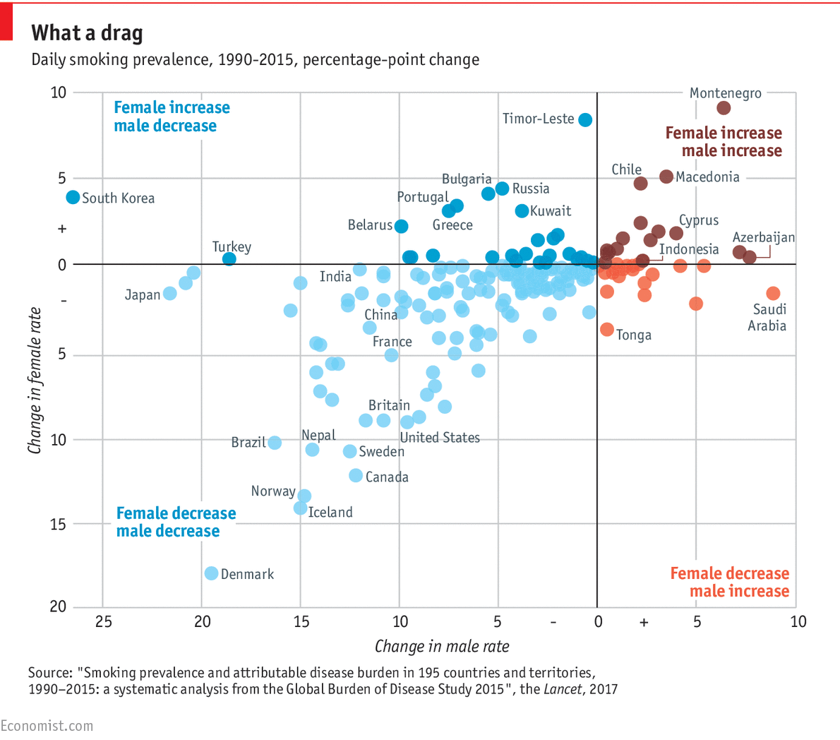
Import data from google sheets I copied and pasted from the orginal article to a google sheets because I didn’t know a faster or easier way. The URL for the data and table of interest is: https://www.thelancet.com/action/showFullTableHTML?isHtml=true&tableId=tbl1&pii=S0140-6736%2817%2930819-X The full article is: https://www.thelancet.com/journals/lancet/article/PIIS0140-6736(17)30819-X/fulltext# Here’s the graph that inspired me: http://cdn.static-economist.com/sites/default/files/imagecache/1872-width/20170415_WOC921.png Here’s the tweet that started it all:
data_from_lancet_key <- gs_key("1I8FKCUhb6WM-vNOL19inNAmWv0Guq_Q9dgdMVsquFOk")## Auto-refreshing stale OAuth token.## Sheet successfully identified: "smoking_prevalence"world_pop_key <- gs_key("1CqdhlwlwXmKA-YEgBhZJECgPqUwv2_PmB2bWpBzyEo0")## Sheet successfully identified: "world_population_world_development_indicators"country_codes_key <- gs_key("1sXQqMu4smGlP7p8vxL6fq7VZSU3Tz-kZB0GtiFFzAKI")## Sheet successfully identified: "countryContinent"data_from_lancet <- gs_read_csv(data_from_lancet_key)## Accessing worksheet titled 'Sheet1'.## Parsed with column specification:
## cols(
## Name = col_character(),
## `SDI level` = col_character(),
## `2015 female age-standardised prevalence` = col_character(),
## `2015 male age-standardised prevalence` = col_character(),
## `Annualised rate of change, female 1990–2015` = col_character(),
## `Annualised rate of change, male 1990–2015` = col_character(),
## `Annualised rate of change, female 1990–2005` = col_character(),
## `Annualised rate of change, male 1990–2005` = col_character(),
## `Annualised rate of change, female 2005–2015` = col_character(),
## `Annualised rate of change, male 2005–2015` = col_character()
## )world_pop_data <- gs_read_csv(world_pop_key, skip = 4)## Accessing worksheet titled 'API_SP.POP.TOTL_DS2_en_csv_v2_162'.## Parsed with column specification:
## cols(
## .default = col_double(),
## `Country Name` = col_character(),
## `Country Code` = col_character(),
## `Indicator Name` = col_character(),
## `Indicator Code` = col_character()
## )## See spec(...) for full column specifications.country_codes <- gs_read_csv(country_codes_key)## Accessing worksheet titled 'countryContinent'.## Parsed with column specification:
## cols(
## country = col_character(),
## code_2 = col_character(),
## code_3 = col_character(),
## country_code = col_double(),
## iso_3166_2 = col_character(),
## continent = col_character(),
## sub_region = col_character(),
## region_code = col_double(),
## sub_region_code = col_double()
## )Cleaning of my data
world_pop_data <- clean_names(world_pop_data)

data_clean <- clean_names(data_from_lancet)

#make sdi_level a factor from a character
data_clean$sdi_level %<>% factor

#separate point values from confidence intervals
data_2_tidy <- data_clean %>% separate(x2015_female_age_standardised_prevalence, into = c("female_prevalence_2015", "female_confidence_interval"), " ", extra = "merge") %>% separate(x2015_male_age_standardised_prevalence, into = c("male_prevalence_2015", "male_confidence_interval"), " ", extra = "merge")
#replace middle dot with period
data_2_tidy$female_prevalence_2015 <- gsub("·", ".", data_2_tidy$female_prevalence_2015)

data_2_tidy$male_prevalence_2015 <- gsub("·", ".", data_2_tidy$male_prevalence_2015)

#repeating prior two steps for other columns
data_2_tidy_all_columns <- data_2_tidy %>% separate(annualised_rate_of_change_female_1990_2015, into = c("female_1990_2015", "female_1990_2015_confidence_interval"), " ", extra = "merge") %>% separate(annualised_rate_of_change_male_1990_2015, into = c("male_1990_2015", "male_1990_2015_confidence_interval"), " ", extra = "merge") %>% separate(annualised_rate_of_change_male_1990_2005, into = c("male_1990_2005", "male_1990_2005_confidence_interval"), " ", extra = "merge") %>% separate(annualised_rate_of_change_male_2005_2015, into = c("male_2005_2015", "male_2005_2015_confidence_interval"), " ", extra = "merge") %>% separate(annualised_rate_of_change_female_1990_2005, into = c("female_1990_2005", "female_1990_2005_confidence_interval"), " ", extra = "merge") %>% separate(annualised_rate_of_change_female_2005_2015, into = c("female_2005_2015", "female_2005_2015_confidence_interval"), " ", extra = "merge")

#Removing middle dot from other columns
#figure out how to make this happen with lapply or something
data_2_tidy_all_columns$female_1990_2015 <- gsub("·", ".", data_2_tidy_all_columns$female_1990_2015)

data_2_tidy_all_columns$female_1990_2005 <- gsub("·", ".", data_2_tidy_all_columns$female_1990_2005)

data_2_tidy_all_columns$female_2005_2015 <- gsub("·", ".", data_2_tidy_all_columns$female_2005_2015)

data_2_tidy_all_columns$male_1990_2015 <- gsub("·", ".", data_2_tidy_all_columns$male_1990_2015)

data_2_tidy_all_columns$male_1990_2005 <- gsub("·", ".", data_2_tidy_all_columns$male_1990_2005)

data_2_tidy_all_columns$male_2005_2015 <- gsub("·", ".", data_2_tidy_all_columns$male_2005_2015)

#Huge issue and roadblock here. Got great help from R Ladies r-help channel
#dash encoding issue: copy paste from the data did not get intrepreted correctly, so I looked at the unicode for it and then used the code

data_2_tidy_all_columns$female_prevalence_2015 <- as.numeric(data_2_tidy_all_columns$female_prevalence_2015)
data_2_tidy_all_columns$male_prevalence_2015 <- as.numeric(data_2_tidy_all_columns$male_prevalence_2015)


data_2_tidy_all_columns$female_1990_2015 <- as.numeric(gsub('\U2212', "-", data_2_tidy_all_columns$female_1990_2015))

data_2_tidy_all_columns$female_1990_2005 <- as.numeric(gsub('\U2212', "-", data_2_tidy_all_columns$female_1990_2005))

data_2_tidy_all_columns$female_2005_2015 <- as.numeric(gsub('\U2212', "-", data_2_tidy_all_columns$female_2005_2015))

data_2_tidy_all_columns$male_1990_2015 <- as.numeric(gsub('\U2212', "-", data_2_tidy_all_columns$male_1990_2015))

data_2_tidy_all_columns$male_1990_2005 <- as.numeric(gsub('\U2212', "-", data_2_tidy_all_columns$male_1990_2005))

data_2_tidy_all_columns$male_2005_2015 <- as.numeric(gsub('\U2212', "-", data_2_tidy_all_columns$male_2005_2015))


#filter out confidence intervals (not really needed but easier to look at)
data_2_tidy_no_cis <- data_2_tidy_all_columns[, c(-4, -6, -8, -10, -12, -14, -16, -18)]
Adding some population data for possible later analysis
merged_data <- merge(data_2_tidy_no_cis, world_pop_data, by.x = 1, by.y = 1)

merged_data_with_codes <- merge(merged_data, country_codes, by.x = 11, by.y = 3)
```
Analysis to make a version of the Economist Plot
economist_analysis <- data_2_tidy_no_cis %>% mutate(male_estimate_1990 = male_prevalence_2015 / ((1+(male_1990_2015/100))^25)) %>% mutate(change_overall_male = male_prevalence_2015 - male_estimate_1990) %>% mutate(female_estimate_1990 = female_prevalence_2015 / ((1+(female_1990_2015/100))^25)) %>% mutate(change_overall_female = female_prevalence_2015 - female_estimate_1990)

economist_analysis <- economist_analysis %>% mutate(quadrant = case_when(change_overall_male > 0 & change_overall_female > 0   ~ "Both Increased",
                              change_overall_male <= 0 & change_overall_female > 0  ~ "M Decreased, W Increased",
                              change_overall_male <= 0 & change_overall_female <= 0 ~ "M Increased, W Decreased",
                              TRUE                                         ~ "Both Decreased"))
Plotting
plot_6 <- ggplot(economist_analysis, aes(x = change_overall_male, y = change_overall_female, color = quadrant, label = name)) +
  geom_point() +
  theme_minimal() +
  geom_hline(yintercept=0) +
  geom_vline(xintercept=0) +

    geom_text_repel(
    data          = subset(economist_analysis, change_overall_male > 6.5 | change_overall_male < -15 | change_overall_female >= 3.5 | change_overall_female < -10 ),

    segment.size  = 0.1,
    segment.color = "grey50") +

  labs(title = "Change in Men's and Women's Smoking Prevalence from 1990 to 2015", subtitle = "Inspired from Twitter and The Economist", caption = "Data from The Lancet") + labs(x = "Change in Men's Prevalence", y = "Change in Women's Prevalence") + theme(legend.position = "none") + annotate("text", x = 6.5, y = 4, label = "Both up")  + annotate("text", x = -6.5, y = -11, label = "Both down") + annotate("text", x = 5, y = -11, label = "Men up, Women down") +  annotate("text", x = -5, y = 6, label = "Men down, Women up")


plot_6